What Does the White Working Class Want?
Contents
Introduction
I recently finished reading Strangers in Their Own Land, in which Arlie Hochschild profiles Tea Party supporters and activists in Louisianna. She mostly writes about their opposition to government restriction and their embrace of family, community, and G-d. While I was reading, I wondered, what policies does the White Working Class want? Or is their policy preference defined entirely in opposition to government doing anything.
To answer this question, I looked at a dataset from DataForProgress, in which they asked respondents about their preference for a variety of different policies.
knitr::opts_chunk$set(echo = TRUE)
knitr::opts_chunk$set(warning = FALSE)
knitr::opts_chunk$set(message = FALSE)
library(tidyverse)
library(here)
library(fs)
library(janitor)
library(skimr)data = read_csv(here::here('content', 'post_data', 'polls', 'DFP_WTHH_release.csv'))First, I’ll create a race-education variable.
data = data %>%
  mutate(
    education = if_else(educ <= 4, 'No 4-Year College Degree', '4-Year College Degree or Higher')
  )

data$race_education = paste0(data$race, '-', data$education)

data = data %>% filter(race %in% c(1:4))
I want to do a factor analysis on the questionnaire to see if I can group policies together.
factor_item = data %>% select(PATH:SOCIALDOMINANCE_SUPERIOR, POP_3, ICE:POLCORRECT)

factor_item = factor_item %>% mutate_all(~ if_else(. ==6, NA_real_, .))

factor_item = factor_item %>% mutate_all(scale, center = T, scale = T)
library(nFactors)
ev <- eigen(cor(factor_item, use = 'na.or.complete')) # get eigenvalues
ap <- parallel(subject=nrow(factor_item),var=ncol(factor_item),
rep=100,cent=.05)
nS <- nScree(x=ev$values, aparallel=ap$eigen$qevpea)
plotnScree(nS) 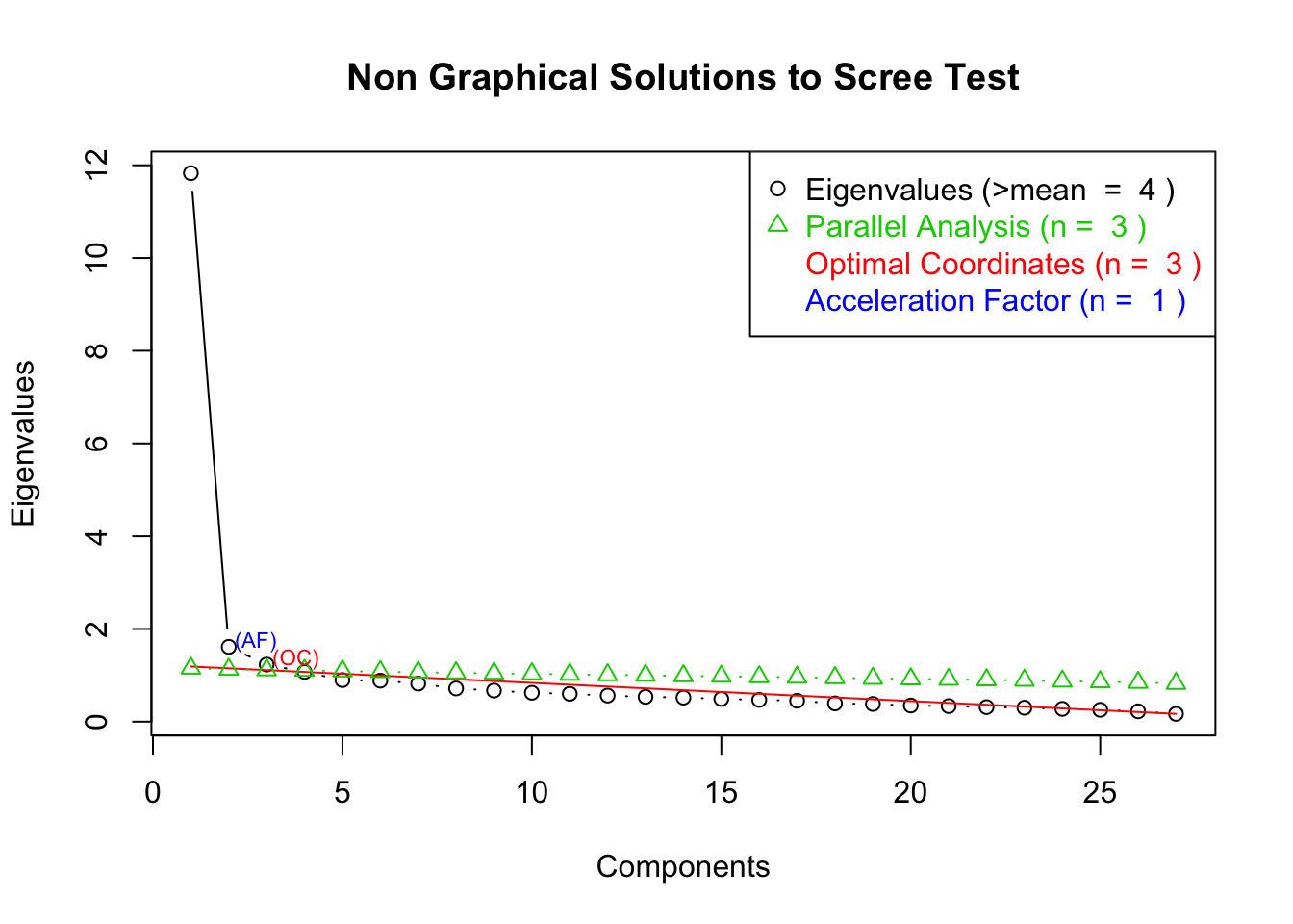
It looks like there are four factors
# Maximum Likelihood Factor Analysis
# entering raw data and extracting 3 factors,
# with varimax rotation
fit <- factanal(na.omit(factor_item), 4, rotation="varimax")
print(fit, digits=2, cutoff=.3, sort=TRUE)
##
## Call:
## factanal(x = na.omit(factor_item), factors = 4, rotation = "varimax")
##
## Uniquenesses:
## PATH BORDER
## 0.87 0.18
## DEPORT SOCIALDOMINANCE_PRIORITIES
## 0.25 0.54
## SOCIALDOMINANCE_NOTPUSH SOCIALDOMINANCE_EQUALIDEAL
## 0.42 0.31
## SOCIALDOMINANCE_SUPERIOR POP_3
## 0.74 0.69
## ICE BAIL_item
## 0.51 0.66
## WELTEST PUBLICINT
## 0.36 0.55
## GREENJOB POLFEE
## 0.48 0.33
## PUBLICGEN BOND
## 0.57 0.46
## FREECOLL WEALTH
## 0.26 0.31
## AVR M4A
## 0.43 0.25
## MARREP MARAM
## 0.77 0.33
## MARLEG YEMEN
## 0.40 0.90
## SOLITARY GUNS
## 0.69 0.43
## POLCORRECT
## 0.41
##
## Loadings:
## Factor1 Factor2 Factor3 Factor4
## BORDER -0.77 -0.33
## DEPORT -0.76
## ICE 0.57 0.32
## WELTEST -0.69 -0.33
## M4A 0.58 0.55
## POLCORRECT 0.62 0.33
## PUBLICINT 0.56
## GREENJOB 0.61
## POLFEE 0.36 0.65
## PUBLICGEN 0.61
## BOND 0.39 0.58
## FREECOLL 0.50 0.63
## WEALTH 0.34 0.69
## SOCIALDOMINANCE_PRIORITIES 0.56
## SOCIALDOMINANCE_NOTPUSH -0.31 -0.30 -0.60
## SOCIALDOMINANCE_EQUALIDEAL 0.34 0.70
## MARAM 0.71
## MARLEG 0.65
## PATH -0.33
## SOCIALDOMINANCE_SUPERIOR -0.43
## POP_3 -0.46
## BAIL_item 0.32 0.36
## AVR 0.44 0.50
## MARREP 0.46
## YEMEN
## SOLITARY 0.39
## GUNS 0.48 0.48 0.33
##
## Factor1 Factor2 Factor3 Factor4
## SS loadings 4.89 4.69 2.35 1.96
## Proportion Var 0.18 0.17 0.09 0.07
## Cumulative Var 0.18 0.35 0.44 0.51
##
## Test of the hypothesis that 4 factors are sufficient.
## The chi square statistic is 1040.2 on 249 degrees of freedom.
## The p-value is 3.52e-97# plot factor 1 by factor 2
load <- fit$loadings[,1:4]
load## Factor1 Factor2 Factor3 Factor4
## PATH -0.32748728 -0.0320810 -0.10583197 -0.07458352
## BORDER -0.76646444 -0.3279173 -0.28814165 -0.21430219
## DEPORT -0.76265056 -0.1998567 -0.29494040 -0.21499691
## SOCIALDOMINANCE_PRIORITIES 0.24802915 0.2759873 0.55679822 0.12791728
## SOCIALDOMINANCE_NOTPUSH -0.30696191 -0.3045940 -0.60471282 -0.15019642
## SOCIALDOMINANCE_EQUALIDEAL 0.24830382 0.3418335 0.69802800 0.14358090
## SOCIALDOMINANCE_SUPERIOR -0.21340927 -0.1071404 -0.42580550 -0.15472208
## POP_3 -0.46270509 -0.1812516 -0.17503672 -0.18589847
## ICE 0.57301828 0.3214573 0.13461294 0.19735587
## BAIL_item 0.29252380 0.3206723 0.14626890 0.36112189
## WELTEST -0.69043955 -0.1372896 -0.19705230 -0.32975948
## PUBLICINT 0.23885675 0.5637251 0.18801240 0.20055373
## GREENJOB 0.18910059 0.6142404 0.25216437 0.21531503
## POLFEE 0.36299450 0.6530744 0.27712740 0.18922597
## PUBLICGEN 0.09890935 0.6051896 0.09921924 0.19870932
## BOND 0.38745693 0.5788993 0.12582616 0.20939481
## FREECOLL 0.50088663 0.6326282 0.21012005 0.20763016
## WEALTH 0.33531263 0.6884247 0.22670662 0.21853054
## AVR 0.44493683 0.4975190 0.26083509 0.23375774
## M4A 0.58239173 0.5463843 0.23848257 0.23337750
## MARREP 0.01703181 0.4560955 0.14693220 0.02587246
## MARAM 0.25028115 0.2315998 0.19832551 0.71411993
## MARLEG 0.29478004 0.2405518 0.17819001 0.65132963
## YEMEN 0.19057439 0.1423934 0.05776742 0.18940542
## SOLITARY 0.38596133 0.2459442 0.13711567 0.27813160
## GUNS 0.48017462 0.4778210 0.32584633 0.07081249
## POLCORRECT 0.62480321 0.3328249 0.27408196 0.09668757So, the four factors are:
- Pro-border wall, pro deportation of undocumented immigrants, against free college, against political correctness
- Against green-jobs, against wealth-tax, and against free college
- Against equality between groups should be ideal
- Against marijuana reform
Let’s create the factor scores
create_factor_vars = function(index){

  fact = rownames(fit$loadings)[abs(fit$loadings[,index]) >= .3]
  reverse_code = rownames(fit$loadings)[(fit$loadings[,index]) <= -.3]
  fact_name = paste0('fact_', index)
  data <<- data %>% mutate_at(reverse_code, function(x) (max(x, na.rm = T) + 1) - x )
  data[[fact_name]] <<- rowMeans(data[,fact], na.rm = T)

}

walk(1:4, create_factor_vars)
And see where the white working class scores relative to everyone else on these measures
- 1 = White
- 2 = Black
- 3 = Hispanic
- 4 = Other
library(ggplot2)
library(ggridges)

data_long = data %>% select(fact_1:fact_4, race_education) %>% gather(key, value, -race_education)


ggplot(data_long, aes(x = value, y = race_education, fill = race_education)) +
  stat_density_ridges(quantile_lines = TRUE, quantiles = c(0.025, .5, 0.975), alpha = 0.7) + facet_wrap(~ key)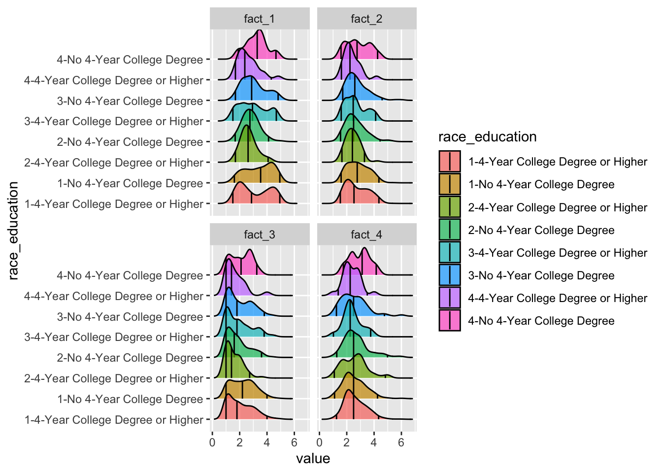
In the above group, the three lines represent the 25th, median, and 75th percentile
The thing that pops out to me is that the White Working Class is drastically different from everyone else – take a look at the medians. They often line up for everyone except the White Working Class.
To summarise, they are
- More Pro-border wall, pro deportation of undocumented immigrants than everyone else
- More against green-jobs and a wealth tax than everyone else
- More against equality between groups should be ideal than
- In line with almost everyone else on marijuana reform.
Author Sam Portnow
LastMod 2018-09-07